A Benchmark Evaluation of Metrics for Graph Query Performance Prediction
- Queries are the foundations of data intensive applications. In model-driven software engineering (MDSE), model queries are core technologies of tools and transformations. As software models are rapidly increasing in size and complexity, most MDSE tools frequently exhibit scalability issues that decrease developer productivity and increase costs. As a result, choosing the right model representation and query evaluation approach is a significant challenge for tool engineers. In the current paper, we aim to provide a benchmarking framework for the systematic investigation of query evaluation performance.
More specifically, we experimentally evaluate (existing and novel) query and instance model metrics to highlight which provide sufficient performance estimates for different MDSE scenarios in various model query tools. For that purpose, we also present a comparative benchmark, which is designed to differentiate model representation and graph query evaluation approaches according to their performance when using large models and complex queries.
Authors: Benedek Izsó, Zoltán Szatmári, Gábor Bergmann, Ákos Horváth and István Ráth
Case Study Overview
The benchmark uses a domain-specific model of a railway system that contains most typical class diagram constructs. This metamodel will be instantiated, and concepts of the metamodel can be used in queries.
Metamodel
The metamodel is defined as an EMF metamodel:
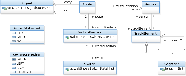
A train route can be defined by a set of sensors between two neighboring signals. The state of a signal can be stop (when it is red), go (when it is green) or failure. Sensors are associated with track elements, which can be a track segment or a switch. The status of a switch can be left, right, straight or failure. A route can have associated switch positions, which describe the required state of a switch belonging to the route. Different route definitions can specify different states for a specific switch.
Metrics
The following metrics were defined to characterize queries and models.
| Type | Name |
|---|---|
| Model only | countNodes |
| countEdges | |
| countTriples | |
| countTypes | |
| avgOutDegree | |
| avgInDegree | |
| maxOutDegree | |
| maxInDegree | |
| Query only | numParameters |
| numVariables | |
| numEdgeConstraints | |
| numAttrChecks | |
| nestedNacDepth | |
| Combined | countMatches |
| selectivity | |
| absDifficulty | |
| relDifficulty |
Model only metrics
- countNodes: Number of instance nodes of the graph model.
- countEdges: Number of instance edges of the model.
- countTriples: The sum of countNodes and coundEdges.
- countTypes: Number of object and relation types.
- avgOutDegree: Average outdegree of nodes.
- avgInDegree: Average indegree of nodes.
- maxOutDegree: Maximum outdegree of nodes.
- maxInDegree: Maximum indegree of nodes.
Query only metrics
- numParameters: Number of query parameters to be returned.
- numVariables: Number of variables in a query.
- numEdgeConstraints: Nunber of relation type constraints.
- numAttrChecks: Number of attribute check expressions.
- nestedNacDepth: The maximum level of nested negations.
Hyprid (model and query) metrics
- selectivity: Number of matches divided by the number of model elements.
- absDifficulty: Sum( ln(1+|c|) ), where |c| is the number of ways a c constraint can be satisfied.
- relDifficulty: Sum( ln(1+|c|) )-ln(1+countMatches)
Query series
Six query series were defined, where in each series queries are scaled in (at least) one query metric. The following table summarizes what is the complexity of the defined series:
| Query series | numParameters | numVariables | numEdgeConstraints | numAttrChecks | nestedNacDepth |
|---|---|---|---|---|---|
| Param | 1-5 | 8 | 8 | 0 | 0 |
| ParamCircle | 1-5 | 6 | 6 | 0 | 0 |
| Locals | 1 | 3-7 | 6 | 0 | 0 |
| Refs | 1 | 5 | 4-7 | 0 | 0 |
| Checks | 1 | 5-11 | 4-10 | 0-6 | 0 |
| Neg | 2-6 | 3-11 | 1-5 | 1 | 0-10 |
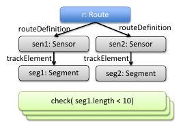
Param and ParamCircle
The following figure depicts the Param, and the less complex ParamCircle patterns graphically:
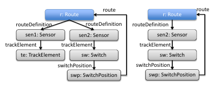
The query body is the same for all patterns in this series, but the first query returns only routes (filled with blue), then the next query adds sen2, then sw, etc.
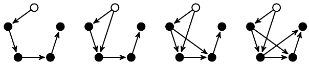
Locals
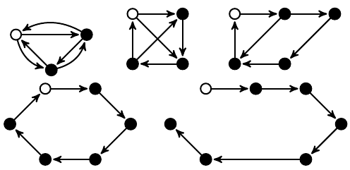
The five patterns of the locals series depicted above. Circles represent object type constraints, while edges the relation type constraints. Unfilled circles show the returned parameter. In all cases there are 6 edge constraints, and the local variables are scaled from 3 up to 7 elements.
Refs
The Refs series displayed similarly as the Locals series above. However, here the number of local variables are the same (five), and the number of reference constraints varying starting from four, up to seven.
Checks
The type constraints of the Checks queries are the same, but a new check constraint is added to each query, thus the number of attribute checks are ranging from zero to four. Here, the filters are done based on the length and year value of seg1 and seg2.
Neg

For this query, at the lowest level a segment is selected with length less than ten. Next, each new query matches a new segment, and calls the previous pattern negatively. This way the number of nested negations are scaled from zero to five.
Instance model generation
The following table displays characteristics and metrics of generated instance models:
| Model Family | Model structure | countNodes | countEdges | countTriples | countTypes | avgOutDegree | avgInDegree | maxOutDegree | maxInDegree |
| A | Regular | 63289 | 1646386 | 1811752 | 7 | 26.01 | 26.01 | 63288 | 44 |
| A | Binomial | 63289 | 1649179 | 1814545 | 7 | 26.06 | 26.06 | 63288 | 69 |
| A | HyperGeo | 63289 | 1646386 | 1811752 | 7 | 26.01 | 26.01 | 63288 | 74 |
| A | Scalefree | 63289 | 1660033 | 1825399 | 7 | 26.23 | 26.23 | 63288 | 10390 |
| B | Regular | 3954 | 102839 | 113170 | 7 | 26.01 | 26.01 | 3953 | 44 |
| B | Binomial | 3954 | 102984 | 113315 | 7 | 26.05 | 26.05 | 3953 | 64 |
| B | HyperGeo | 3954 | 102839 | 113170 | 7 | 26.01 | 26.01 | 3953 | 69 |
| B | Scalefree | 3954 | 96029 | 106360 | 7 | 24.29 | 24.29 | 3953 | 918 |
| C | Regular | 120001 | 1040000 | 1280001 | 7 | 8.67 | 8.67 | 120000 | 13 |
| C | Binomial | 120001 | 1041323 | 1281324 | 7 | 8.68 | 8.68 | 120000 | 30 |
| C | HyperGeo | 120001 | 1040000 | 1280001 | 7 | 8.67 | 8.67 | 120000 | 29 |
| C | Scalefree | 120001 | 1012858 | 1252859 | 7 | 8.44 | 8.44 | 120000 | 8929 |
Model family
For the benchmark three model families (A, B and C) were generated. Models of the A family are large models (containing 1.8M elements), and have relatively large (~26) average outdegree of nodes. The B model family contains smaller models (with 113k elements), but have the same ~26 average outdegree of nodes. For the C family, the average outdegree was lowered (to ~8), but the size of the models are larger, containing 1.2M elements.
Model structure
The distribution of typed edges for a given object type was also considered. Four distributions were generated: regular, binomial, hyper geometric and scale-free. Such distributions were analyzed, for example social networks or molecular structures show scale-free characteristics. For example the binomial model structure means: the number of outgoing and incoming edges of nodes with a fixed type shows binomial distribution for a given relation type.
Benchmark description
The benchmark simulates a typical model validation scenario in a model-driven system development process. A benchmark scenario is built up from well defined phases, executed (and measured) them one after another in the following order:
Phases:
- Read: In the first phase, the previously generated instance model is loaded from hard drive to memory. This includes parsing of the input, as well as initializing data structures of the tool. The latter can consume minimal time for a tool that performs only local search, but for incremental tools indexes or in-memory caches are initialized.
- Check, re-check: In the check phases the instance model is queried for invalid elements. This can be as simple as reading the results from cache, or the model can be traversed based on some index. Theoretically, cache or index building can be deferred from the read phase to the check phase, but it depends on the actual tool implementation. To the end of this phase, erroneous objects must be available in a list.
Technical details
Measurement environment
The exact versions of the used software tools and parameters of the measurement hardware are shown in the following list.
- Measured tools
Tool Model lang. Query lang. Tool version Java EMF Java 6.0 EMF-IncQuery EMF IQPL 0.7.0 Sesame RDF SPARQL 2.5.0 - Environment
- Eclipse: Juno
- Java version 1.6
- Ubuntu precise 64 bit
- Hardware
- CPU: Intel(R) Xeon(R) CPU L5420 @2.50 GHz
- 32 GB RAM
Measurement procedure
The benchmark procedure is implemented as Java applications (or Eclipse Application where necessary). The binaries are independent (i.e.: jar-s are not included which are not dependencies), and the tests are executed in different JVMs in a fully automated way.
To reproduce our measurement please follow these steps:
- Setup the 64 bit Linux environment with Java and Eclipse
- Checkout the metamodel project into an Eclipse workspace from SVN:
- In a runtime Eclipse (where the metamodel plug-in is loaded) checkout the benchmark projects from SVN:
- hu.bme.mit.Train.common
- hu.bme.mit.Train.constraintCheck
- hu.bme.mit.Train.constraintCheck.java2
- hu.bme.mit.Train.constraintCheck.incQuery.0.6
- hu.bme.mit.Train.constraintCheck.incQuery.0.6.patterns
- hu.bme.mit.Train.constraintCheck.sesame
- Checkout the instance model project holder from SVN:
- hu.bme.mit.Train.InstanceModels
- hu.bme.mit.Train.generatorProb
- hu.bme.mit.Train.generatorProb.incQuery
- In the RuntimeConstants.java file of the hu.bme.mit.Train.common project set workspacePath to point to the workspace containing the hu.bme.mit.Train.InstanceModel project.
- Instance models can be generated automatically with the generator above. After the generation, there must be an EMF model in files e.g.: hu.bme.mit.Train.InstanceModels/models/*.concept.
- Testcases must be exported to runnable JAR files (Java and Sesame) or to Eclipse products (for EMF-IncQuery).
- The whole benchmark can be run automatically with the help of scripts in hu.bme.mit.Train.tests.nativ. (See scripts/runTestsBA.sh.)
To calculate metrics on EMF models, use the hu.bme.mit.metrics project from SVN.
Measurement results
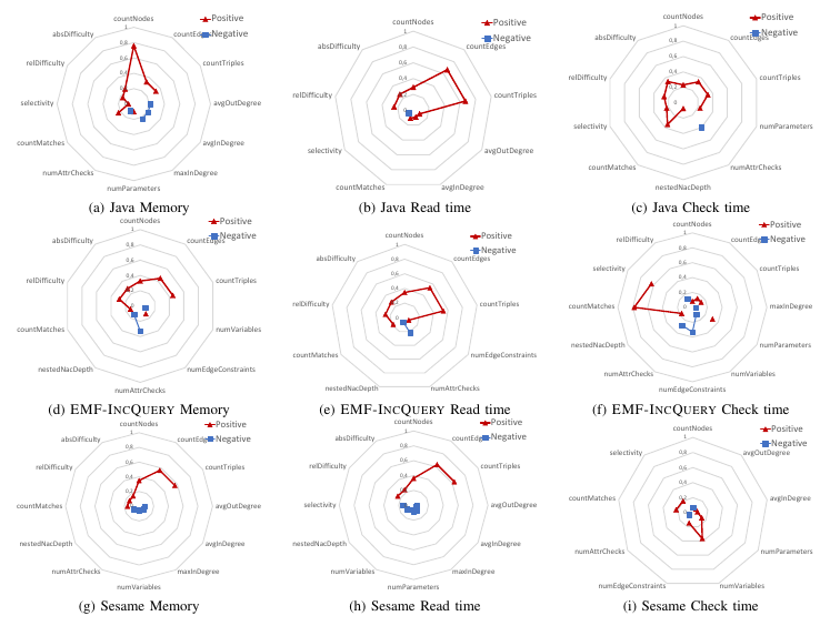
The measurements were performed ten times, the raw results can be downloaded here. The metrics are exported into CSV (calculated automatically by our metrics analyzer) are exported into CSV, and the measured benchmark results into another file. The correlation analysis was performed by this R script, which results were fed into Excel to generate the following spider charts. These diagram show Kendall's tau rank correlation with the measured value (memory, read, check) for a given tool, where the p significance value is less than 0.001.
For the tabular overview see the following figure (available in greater resolution), where tools are listed in one line, and phases in columns.