Incremental Pattern Matching for the Efficient Computation of Transitive Closure
Introduction
Pattern matching plays a central role in graph transformations as a key technology for computing local contexts in which transformation rules are to be applied.
Incremental matching techniques offer a performance advantage over the search-based approach, in a number of scenarios including on-the-fly model synchronization, model simulation, view maintenance, well-formedness checking and state space traversal. However, the incremental computation of transitive closure in graph pattern matching has started to be investigated only recently. In the paper, we propose multiple algorithms for the efficient computation of generalized transitive closures. As such, our solutions are capable of computing reachability regions defined by simple graph edges as well as logical binary relationships defined by graph patterns, that may be used in a wide spectrum of modeling problems.
We also report on experimental evaluation of our prototypical implementation, carried out within the context of a stochastic system modeling case study.
How to obtain the source code
Download an Eclipse Helios (3.6) Modeling product from http://www.eclipse.org.
Obtain the VIATRA2 framework from the nightly update site: http://viatra.inf.mit.bme.hu/update/nightly/
Download the following source plug-ins:
- org.eclipse.viatra2.gtasm.patternmatcher.incremental and org.eclipse.viatra2.gtasm.patternmatcher.incremental.rete plug-ins from https://viatra.inf.mit.bme.hu/svn/core/branches/rete_tranzitivlezart/
- org.eclipse.viatra2.emf.incquery.base.itc from https://viatra.inf.mit.bme.hu/svn/incquery/trunk/runtime/
- org.eclipse.viatra2.gui.stochsim, org.eclipse.viatra2.gtasm.stochastic and org.eclipse.viatra2.console.stochsim plug-ins from https://viatra.inf.mit.bme.hu/svn/stochsim/trunk/
- StructNet from https://viatra.inf.mit.bme.hu/svn/transformations/collab/trunk/stochasti.... This plug-in contains the demonstrating example for the case study which we used during the performance measurements.
Structure of the StructNet project
- Distributions folder: contains all the necessary xml files to configure the simulation
- ioA: log files will be placed here during simulation
-
snet_generator.vtcl is used to generate sample models for measurements. Three parameters are used for a generation:
- NSCC: number of SCCs in the initial configuration
- NSn: number of super nodes in an SCC in the initial configuration
- NCl: number of client nodes connected to every super node in an SCC
- snet_simplified_gen.vpml: VIATRA2 model space file which contains the meta and instance models. You must specify the path of your StructNet plug-in within your workspace under
- root.StoSimPars.ioPath (for example C:\Users\Default\runtime-stochsim\StructNet).
- snetRules_reduced_optimized.vtcl: conatins the patterns used for the VoIP case study.
How to run the simulation
For more information about how to use the VIATRA2 framework please visit http://wiki.eclipse.org/VIATRA2.
One can run the simulation as a console application or with GUI support in a Runtime Eclipse.
Running the simulation with GUI support
- Create a new Eclipse Application Run Configuration and add all the plug-ins to the config mentioned earlier.
- Run the Application.
- Open the snet_simplified_gen.vpml file (it will appear as an entry in the VIATRA2 Model Spaces view).
- Optionally you can generate an initial model with the snet_generator.vtcl file (after opening press ALT + P and it will be added to the Model Spaces view).
- If you double click on the file inside the Model Spaces view it will run the generator.
- Open the snetRules_reduced_optimized.vtcl file and add it to the Model Spaces view with pressing ALT + P.
- If you right click on the label of the file (inside the Model Spaces view) you can choose 'Run stochastic simulation' from the context menu.
Running the simulation as a console application
- Create a new Eclipse Application Run Configuration and add all the plug-ins to the config mentioned earlier.
- Set the Run a product to 'org.eclipse.viatra2.console.stochsim.stochsim_console' in the Main tab.
- Add program arguments in the following order name_of_vpml_file name_of_vtcl_file name_of_machine (for example snet_simplified_gen.vpml snetRules_reduced_optimized.vtcl snet.snetRules)
- Set the working directory to the StructNet plug-in's folder (for example C:\Users\Default\runtime-stochsim\StructNet).
Detailed measurement results
Please see the attached zip archive, which contains all of the measurement results which we carried out during the experiments with the simulator. The archive contains an Excel file.
Notes on the Excel file:
- sheet named 'base_addlink_0,005': contains all measurements with the rate of addLink rule set to 0,005. The column names are as follows:
- NSCC: number of SCCs in the initial configuration
- NSn: number of super nodes in an SCC in the initial configuration
- NCl: number of client nodes connected to every super node in an SCC
- MAX DEPTH: maximum number of steps per simulation run
- MAX TIME: maximum duration allowed for the simulation run
- TIME: the actual logical time spent during the simulation
- SIM RUNTIME: the runtime of the execution of the simulation
- P_NetworkSize and P_ConnectedOverlayPairs are probes
- CPUTIME_RETE: time spent in the RETE engine
- MAXSIZE: maximum size of the results of the given probe
- AVG: average size of the results of the given probe
- TOTAL INCSCC UPDATE TIME: total time spent during the execution of the IncSCC algorithm's update logic
- INCSCC INIT TIME: total time spent on the initialization of the transitive closure relation with the IncSCC algorithm
- TOTAL_DRED UPDATE TIME: total time spent during the execution of the DRED algorithm's update logic
- DRED INIT TIME: total time spent on the initialization of the transitive closure relation with the DRED algorithm
- AVERAGE NUMBER OF SCCs: the average number of SCCs
- TOTAL_CPUTIME_EXEC: time spent for the simulation itself (does not contain the time spent during the update of RETE)
- P_ConnectedOverlayPairs_LS: the probe was evaluated with the local search algorithm
- sheet named 'base_addlink_2': contains all measurements with the rate of addLink rule set to 2. The column names are the same as in the previous sheet.
- sheet named 'varying_addlink': in these measurements the model size was fixed (NSCC - 20, NSN - 10, NCL - 9) and the rate of addlink was varied from 0,005 to 5.
- The rest of the sheets contains the table and diagram presented in the paper.
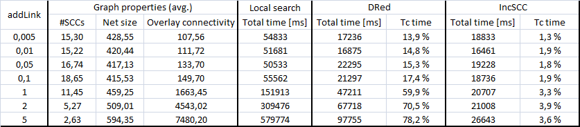
The following table shows the results of the fi rst experiment series. In these measurements we compared the performance of the IncSCC, DRED and local search algorithms. For each value of addLink, we have displayed (i) the values of the probes (as well as the number of strongly connected components) averaged over an entire simulation run; (ii) for each of the three solutions the total execution time and, in case of the incremental algorithms, (iii) the time spent initializing and updating the transitive closure node (expressed as a percentage of total time).
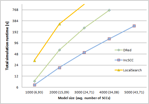
The following figure shows the results of the second experiment series. For each model size on the horizontal axis, we have displayed the average number of SCCs in the model, and on the logarithmic vertical axis the total simulation execution times in case of the three solutions.